SoccerNet Player Re-identification
Last semester as a part of CSE 610 Sports Video Analytics class, we worked on the Soccernet-Player Re-identification challenge. Below are the notes from the work done in this project.
What’s the task of Person Re-identification?
The task of Person Re-identification can be formulated differently leading to multiple definitions. I will start with one which is quite straightforward, and introduce others later.
As name suggests it is all about “Re” identifying the person. More precisely, person Re-identification is a task of
identifying the same person in two time and/or view disjoint frames taken from multiple cameras.
Below is an image from person re-identification dataset called Market-1501(Zheng et al., 2015). It contains in
total 8 sequence of images(3 sequences in first two rows and two sequences in the last row. Note, here sequence doesn’t
necessarily mean any order between images, it just is a collection), each image in a sequence is of the same person/identity
taken from multiple views captured by different cameras in a market. The task of person re-identification is to build the
correspondence between images in the same sequence. Also, as can be seen in the last row, there can also be negative
examples i.e. there is either no sufficient information to identify the person or there’s no more images to retrieve
(only single reference image). Based on requirements of a task at hand, output in such cases could be different e.g. “none”
if similarity score/ other metric is below some reasonable threshold value.

Having gone over what person re-identification is, player re-identification is self-explanatory : person re-identification
done for players in particular sports.
Mostly all publicly available person/player re-identification datasets have cropped images of players from image frames in the video. These videos can be from different geographic locations and timestamps, captured from multiple cameras with dissimilar views/orientations. Although timestamps are different, difference is smaller (in minutes or less). Multiple camera views pose a challenge because the views are disjoint, temporal distance between images is not constant, lighting conditions and backgrounds are different.
Given such dataset, you will find some standard definitions in literature which I will introduce here.
- Anchor/Query Image : An image of the target player to be re-identified.
- Action frame : A frame from which an anchor image is captured. In case of SoccerNet dataset, action signifies some interesting
event in the soccer e.g. a goal. All the frames in the
video for that action are grouped together and used for evaluation as these frames are temporally closer.
- Reference frame: All other frames (can be from same or different action) in the dataset except the action
frame.
- Gallery set: Nothing fancy, it simply is a set of all reference frames / bounding boxes(likely have different views/timestamps).
- Positive Image: An image of the same identity as that in the anchor image.
- Negative Image: An image which doesn’t have the same identity as that in the anchor image.
Below is the illustration of Soccernet-v3 dataset -

Let’s say above image is divided into four parts by two dotted lines. Top left corner is an action frame, most likely a goal.
After that, in top right you have reference frames named as replay frames; notice the small temporal distance
between action and replay frames. In the lower-left part of the image, 18 bounding boxes are captured, each will be used as
(possible) query image, and all the 37 bounding boxes captured from the reference images will form a gallery, shown in the
lower right part. In some cases, such as the bottom-most image of a referee in the queries doesn’t have any matching image
in the gallery set, then it will be moved to gallery set to create a distraction. Having taken a look at some images
in the dataset, take a minute to think about the challenges I mentioned in the dataset such as difference in background,
resolution and size.
So in summary, an anchor image is taken from action frames; positive images and negative images are taken from reference frames/gallery set. You are given an anchor image, your model needs to find the Positive image from the Reference images. With above description you could also formulate the problem of re-identification in terms of image retrieval based on metric learning. I will talk more about metric learning in later sections.
State-of-the-Art methods of Re-identification
Current methods of player re-identification mainly focus on two ways - one is to get high quality discriminative features and other is to define the distance metric which can be used as a loss for learning task effectively. I will talk briefly about the prior as it aligned with the requirements of the class. While learning the features from the images, it is important to work on relatively similar scale of the images. In more open-world settings, distance of objects from the camera is different, and so ae there sizes in the image; although to some extent it is taken care by cropping the image and resizing the images to same size, it is important to construct features from different scales in an image. One of such methods exploring the ideas of multiple scales is from the authors of OSNET(Zhou et al., 2019).OsNET was also SOTA method in SoccerNet baselines which gave the best results. One of the other methods that we reviewed was recent addition to SOTAs, a transformer based re-identification model - TransReid. Let me describe both OSNET and TransReid in following sections.
1. Omni-Scale Feature Learning for Person Re-Identification (OSNET) (Zhou et al., 2019)
Authors of this paper argue that to match the people, small local features (e.g. shoes,
purse etc.) and relatively larger global features (e.g. whole body appearance) are equally important. Therefore, such discriminative
features should be omniscale, defined as the combination of variable homogeneous scales and heterogeneous scales,
each of which is composed of a mixture of multiple scales.
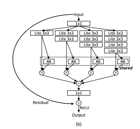
Authors propose a novel CNN architecture OSNET. The main idea is to have multiple CNN streams with different receptive fields so that the multiscale features can be learnt. At last, resulting multiscale feature maps from each stream are fused by weighted aggregation gate (AG). The AG is a mini-network sharing parameters across all the CNN streams. With the trainable AG, the generated channel-wise weights become input-dependent, hence the dynamic scale fusion. There are some more ideas adapted in this paper such as depth-wise convolutions to make the module light-weight. For more detailed understanding reader is advised to review OSNET paper (Zhou et al., 2019).
2. TransReid: Transformer-based Object Re-Identification (He et al., 2021)
One of the other methods which although, doesn’t directly encode multiscale features it does address main problems with CNN based
Re-ID methods. I have seen TransReid perform quite well in the task of player re-identification, which should come with no
surprise as Transformer based models are performing better and better stacking up hundreds of submissions in the top
conferences these days.
There are two main problems with the traditional CNN based approaches of re-identification - 1. CNN based methods focus on small discriminative features due to a Gaussian distribution of effective receptive fields. 2. Down-sampling operators of CNN reduce the spatial dimension of the feature-map (as you would also see that this was one of the motivations for us to use Layer-wise similarity discussed in the later section).
Authors of TransReid propose to address these issues -
Use of attention captures long range dependencies as complete global information is available at each layer despite its
depth. Without down-sampling operators, transformers can keep more detailed information. To further add robust features authors
introduce two modules -
- Jigsaw patches module : As with vision transformer, (Dosovitskiy et al., 2020) the image is split into fixed sized patches and attention based mechanism is used to learn the features. This module attempts to rearrange the patch embeddings via shift and shuffle operations and regroup them for further feature learning. This enables robustness in the learned features and also expands on long-range dependencies.
- Side information embedding : In many of the re-identification datasets we have non-visual information which can not be processed by purely CNN based model. Therefore, there is no way of addressing data bias brought by cameras or viewpoints. This module, similar to position encoding in vision transformer, uses learnable 1D embeddings to encode side information suh as camera and view metadata.

For more detailed treatment of TransReid reader is advised to review TransReid paper (He et al., 2021)
Appearance and Pose as discriminative features
Motivation:
As compared to the task of person re-identification, the task of player re-identification is significantly challenging. Many methods base their model on
appearance as discriminative feature to learn the metrics, but in case of players, appearance of almost all is similar - for example in a game of
football the general physique of all the players would be on average similar. Almost all players from same team will wear similar jersey, exception being
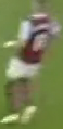
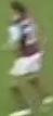
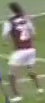
goal-keepers, but there is only one goalkeeper in a team on the field. Now, you might be able to identify player based on their jersey numbers but remember we have to
re-identify players from different camera views, and it is more likely than not that the jersey numbers are either not visible in the given view or too obscure to
even be detected let alone be identified as can be seen from below pictures.
Therefore, appearance features alone are not sufficient. It is also evident from the difference in the performance of the SOTA
methods such as OSNET on person re-identification vs player re-identification.
| Dataset | mAP (%) | Rank-1 (%) |
|---|---|---|
| Person re-identification (Market1501) | 81 | 93.6 |
| Player re-identification (SoccerNet-v3) | 61.6 | 51.2 |
One of the main difference we identified in traditional person re-identification datasets and SoccerNet dataset is that temporal distance between anchor image and reference images in case of SoccerNet dataset is much smaller than that of person re-identification datasets. Which means a player in anchor image and the same player in (positive) reference images is likely to have similar body posture. Also, in almost every team-sport, based on the role of a player in overall game, there are distinct moves that they do at a given time. Posture of players therefore, could be used as additional discriminative feature to guide the task of metric learning. This was one of the main ideas that we implemented in the project.
Methodology:
We need to extract both posture features and appearance features from the input image; We use two-stream model where one
stream is called as appearance extractor which works on extracting the appearance features from the images, and second stream
called as part/pose extractor works on extracting the pose related features from the images. We use RESNET-50 as appearance extractor
and sub-model of openpose as pose-extractor. At the end we need to combine both the appearance and pose features to calculate
the final loss. We use (compact) bi-linear pooling to pool the features from both the streams. Our choice of pose extractor and pooling
has been adapted from Part-aligned bilinear pooling for re-identification paper(Suh et al., 2018).
Below image shows the two-stream extractor -

Note that we use two losses, first is Triplet loss as a similarity loss which will be explained in detail in a later section. Another is an identity loss, this is nothing but a traditional cross-entropy loss used in classification tasks. It is formally given as,
\[L = \frac{1}{m} \sum_{i=1}^m y_i \dot{} \log{\hat {y}_i}\]OpenPose:
Let me briefly describe main concepts in OpenPose and the sub-model that we use in our work.
OpenPose(Cao et al., 2018) is the first open-source realtime system for multi-person
2D pose detection, including body, foot, hand, and facial keypoints (total 135 keypoints).
Authors of OpenPose: Ginés Hidalgo (left) and Hanbyul Joo (right) in front of the CMU Panoptic Studio. image source
There are mainly two approaches in multi-person 2D human pose detection -
- Top-down approach - In top-down approach, a single person is detected first, and then the pose is estimated for every such detection.
- Bottom-up approach - On the contrary, in bottom-up approach, local features (such as body parts) are detected and associated with each other to get the global context/information about complete pose.
OpenPose is based off Bottom-up approach. Figure below visualizes the complete pipeline of the OpenPose.
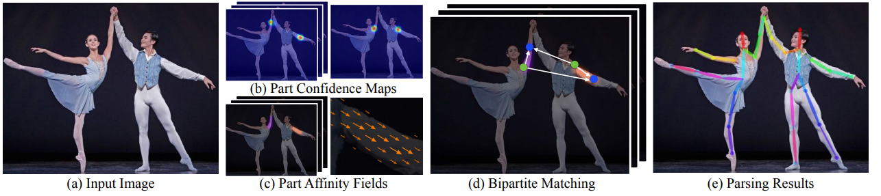
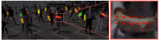
OpenPose takes in 2D color image of size $H \times W$ as input (Fig. a) and produces anatomical key points on each person in the image as output (Fig. e). First, feed-forward network predicts set of confidence maps $S$ of body parts (Fig. b) and set of 2D vector fields $L$ called as part affinity fields (PAF), which encode degree of association between body parts (Fig. c). The set $S=(S_1, S_2, …, S_J)$ has $J$ confidence maps, one per part, where $S_j \in \mathbb{R}^{w \times h}$, $j \in {1 . . . J}$. The set $L=(L_1,L_2, …,L_C )$ has $C$ vector fields one per limb (including face, although technically it’s not a limb) where $L_c \in \mathbb{R}^{w \times h \times 2}$, $c \in {1, ..C}$. Once all the PAFs and confidence maps are identified, bipartite matching does the association and the result is 2D key-points for all people in the image (Fig. d). Note that each image location in L encodes a 2D vector as shown in the below figure.
As stated earlier, we only need a sub-model of the OpenPose, particularly, the part until it calculates the final part confidence features which we use for bi-linear pooling with appearance features. Multi-stage architecture of OpenPose is given in the below figure, where first stages predict PAFs and later stages predict the part confidence maps.
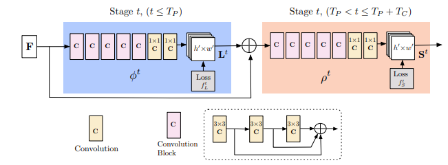
First, image is fed into pretrained VGG-19, which gives the feature maps $F$ that is input to the first stage and outputs the first PAF. In each subsequent stage, the predicted PAF from the previous stage and the original image feature map $F$ are concatenated and used to produce the refined predictions. Formally first PAF $L^1$ is calculated as,
\[L^1 = \phi^1(F)\]Subsequent PAFs are calculated as,
\[L^t = \phi^t(F, L^{t-1}), \forall 2\le t \le T_p\]where, $\phi^t$ refers to CNNs inference at stage $t$. After total of $T_p$ PAF stages, last PAF is given as input to next stage for estimating part confidence map. First stage only takes $L^{T_p}$ and $F$ as inputs, i.e.
\[S^{T_p} = \rho^t(F, L^{T_p}), \forall t=T_p\]whereas subsequent stages take $L^{T_p}$, $F$ and $S^{T-1}$ as inputs, i.e.
\[S^{t} = \rho^t(F, L^{T_p}, S^{t-1}), \forall T_p \lt t \le T_p + T_c\]where $T_c$ is number of confidence map estimation stages and $\rho^t$ is CNNs inference at stage $t$ which estimates part confidence map. We initialize the pose-extractor with OpenPose pretrained on COCO dataset. Note that we do not need ground-truth pose estimations of SoccerNet-v3 because we only optimize the re-identification loss.
We trained the model for 50 epochs, with 32 batch size and 10% percentage (of unique person IDs) of SoccerNet-V3 data. As can be seen in the below table we were able to surpass the OSNET performance and other baselines. Adding Layer-wise similarity (described in later section) and adding channel and/or spatial attention could further increase the performance.
| Model | mAP (%) | Rank-1 (%) |
|---|---|---|
| OSNET | 61.6 | 51.2 |
| inceptionv4 | 46.7 | 32 |
| RESNET50mid | 46.5 | 31.7 |
| RESNET50 | 46.7 | 32.8 |
| Ours | 63.7 | 52.9 |
Layer-wise similarity
Before diving into the idea of layer-wise similarity, let me talk little about the metric learning and similarity loss first. Metric learning is a task of machine learning in which the loss to be minimized is a distance between data points. Similarity loss in this context is any type of loss which measures the similarity between images (anchor and any other image). Triplet loss is one of the most frequently used metric learning losses in the re-identification. It is formally defined as,
$$ L = max(d(a, p) - d(a, n) + \delta, 0) $$ where $d$ is any distance metric such as euclidean or manhattan distance. We use $L2$ distance. $a$ is an anchor image, $p$ is a positive image, $n$ is a negative image. $\delta$ is a margin. Minimizing the triplet loss in a training has an effect of pushing away negative samples and bringing the positive samples closer simultaneously, as illustrated in the below image.

RESNETs have been champions in almost all computer vision tasks from much of their inception. Unsurprisingly, RESNET was also
implemented in official SoccerNet reidentification developement kit. Although, RESNET’s
performance was no way near the state-of-the-art methods their wide use steered us to use it as a backbone model to build upon.
For the reasons stated earlier it was desired that we look at what features in the image RESNET was focusing on. Below is
activation map of some of the middle layers of the RESNET.

In every part out of 6 parts of the activation map image above, there are total of three smaller images. First is a bounding box image which is an input to the respective RESNET layer, second is output (activation map) of the respective RESNET layer and the last is superimposition of activation map on the input to highlight the feature each layer is focusing on. As can be seen, the output/last layer of RESNET was focusing on small spatial features such as shoes in this case, although features such as jersey number were detected in earlier layers. This is one of the drawbacks of CNN based reid models where pooling and strided convolutions reduce the size of output feature maps. Therefore, the idea was to use detected features at every layer in the model to calculate the similarity loss. Doing so would steer model to recognize image as a positive image if not only final feature-maps but also feature-maps at middle layers of the model are largely similar (and vice-versa) to respective feature-maps of the anchor image.
Below image illustrates the design of the layer wise similarity in the model,

We add FC layers at the end of the RESNET layers to be taken for calculating the layer-wise similarity. We calculate the similarity loss at the output of the FC layers. The total loss is addition of constituent losses at each layer. The number of FC layers and which layers of RESNET to use is chosen based on the validation. Results on the 10% Soccernet data with batch size of 32 with RESNET as backbone show 3.2% improvement in Rank-1 accuracy and 3.7% increase in mAP.
| Model | mAP (%) | Rank-1 (%) |
|---|---|---|
| Resnet Baseline | 46.7 | 32.8 |
| Layerwise similarity | 50.4 | 36.2 |
One of the further areas of exploration is to utilize pose features which are view invariant such as mentioned in View-Invariant Probabilistic Embedding for Human Pose (Sun et al., 2019). Also, such positional embedding can be effectively utilized with SIE module of TransReid.
Ok, that’s it.
Finally, I am grateful to the support of Dr. David Doermann - for providing resources required for this project. This project-work was done with equal contributions from Mahesh Bhosale and Abhishek Kumar.
Resources:
SoccerNet challenge page
SoccerNet development kit
Our Github Repo
Our report
References
- Zheng, L., Shen, L., Tian, L., Wang, S., Wang, J., & Tian, Q. (2015). Scalable Person Re-identification: A Benchmark. Computer Vision, IEEE International Conference On.
- Zhou, K., Yang, Y., Cavallaro, A., & Xiang, T. (2019). Omni-Scale Feature Learning for Person Re-Identification. ICCV.
- He, S., Luo, H., Wang, P., Wang, F., Li, H., & Jiang, W. (2021). TransReID: Transformer-based Object Re-Identification. arXiv. https://doi.org/10.48550/ARXIV.2102.04378
- Dosovitskiy, A., Beyer, L., Kolesnikov, A., Weissenborn, D., Zhai, X., Unterthiner, T., Dehghani, M., Minderer, M., Heigold, G., Gelly, S., Uszkoreit, J., & Houlsby, N. (2020). An Image is Worth 16x16 Words: Transformers for Image Recognition at Scale. arXiv. https://doi.org/10.48550/ARXIV.2010.11929
- Suh, Y., Wang, J., Tang, S., Mei, T., & Lee, K. M. (2018, September). Part-Aligned Bilinear Representations for Person Re-Identification. Proceedings of the European Conference on Computer Vision (ECCV).
- Cao, Z., Hidalgo, G., Simon, T., Wei, S.-E., & Sheikh, Y. (2018). OpenPose: Realtime Multi-Person 2D Pose Estimation using Part Affinity Fields. CoRR, abs/1812.08008. http://arxiv.org/abs/1812.08008
- Schroff, F., Kalenichenko, D., & Philbin, J. (2015). FaceNet: A unified embedding for face recognition and clustering. 2015 IEEE Conference on Computer Vision and Pattern Recognition (CVPR), 815–823. https://doi.org/10.1109/CVPR.2015.7298682
- Sun, J. J., Zhao, J., Chen, L.-C., Schroff, F., Adam, H., & Liu, T. (2019). View-Invariant Probabilistic Embedding for Human Pose. CoRR, abs/1912.01001. http://arxiv.org/abs/1912.01001